LinStereo: Linear-Complexity Global Attention for Multi-Scale Iterative Stereo Matching

Wang, Yiran; Turner, Oliver; Ila, Viorela

Drag to reveal

One frozen model, many domains, zero fine-tuning. Drag the handle: the stereo input on one side, LinStereo's dense disparity on the other — the same network across street scenes, indoor and outdoor benchmarks, and underwater footage it has never seen.

LinStereo predicted disparity (turbo colormap)

Input

LinStereo disparity

A single LinStereo model — frozen Depth Anything V3 backbone, trained on SceneFlow only — runs zero-shot across all six datasets, from KITTI street scenes to real underwater SQUID footage it was never trained on. Black = no ground truth.

28%↓

AbsRel — TartanAir-UW ocean

26%↓

AbsRel — SQUID (real underwater)

31%↓

RMSE vs FoundationStereo (TartanAir-UW)

37%↓

Occluded EPE — Middlebury(H)

Competitive with ViT-L systems on standard benchmarks and best on underwater generalization — all from a ViT-B backbone trained on SceneFlow only, with no underwater, real-world, or domain-specific data at any stage.

Abstract

Existing Vision Foundation Model (VFM)-based iterative stereo pipelines under-exploit three information pathways: multi-scale backbone features are collapsed into single-level correlations, geometric priors remain untapped at initialization, and context propagates only locally. These gaps widen under degraded photometric cues, making underwater scenes a stringent generalization test. To address this, we propose LinStereo, built upon Depth Anything V3, whose core is a Position-Aware Linear Attention (PALA) module that replaces local recurrence with global aggregation at linear cost, propagating reliable estimates from well-matched regions into degraded areas while preserving disparity structure. PALA is made effective by two enabling components: Hierarchical Semantic Cost Volumes (HSCV), which supply scale-aligned correlations from the VFM feature hierarchy, and a Depth Prior Initialization (DPI) that converts monocular depth into a metrically calibrated warm start. LinStereo achieves state-of-the-art performance on standard benchmarks and strong cross-domain generalization, particularly on underwater scenes where severe photometric degradation makes stereo matching particularly challenging, surpassing all compared methods with consistent gains (28% AbsRel on TartanAir-UW, 26% on SQUID, a real-world underwater dataset).

Method

Modern VFM backbones encode rich multi-scale semantics and implicit geometry, but the iterative update loop still consumes them through a narrow interface inherited from lightweight encoders. LinStereo closes this gap with a single PALA-centred decoder, enabled by HSCV and DPI — not three independent modules.

LinStereo architecture: frozen Depth Anything V3 backbone feeding Hierarchical Semantic Cost Volumes, Depth Prior Initialization, and the Position-Aware Linear Attention updater. — **Architecture.** A frozen Depth Anything V3 backbone produces, in a single forward pass, multi-scale stereo features and a monocular depth map. The PALA updater replaces the ConvGRU with global linear attention over cost-volume features, using 2D rotary position encoding and an adaptive gating branch.

WHAT to match

HSCV

Hierarchical Semantic Cost Volumes build a per-scale correlation volume from each VFM scale (s ∈ {4,8,16}), kept simultaneously queryable, each with its own 4-level disparity pyramid.

WHERE to start

DPI

Depth Prior Initialization turns DA3's affine-invariant monocular depth into a metric disparity warm start via SIFT-based scale–shift alignment — refinement no longer starts from zero.

HOW to refine

PALA

Position-Aware Linear Attention aggregates global context at O(N) per iteration, propagating reliable disparity from textured regions into degraded, textureless areas.

01

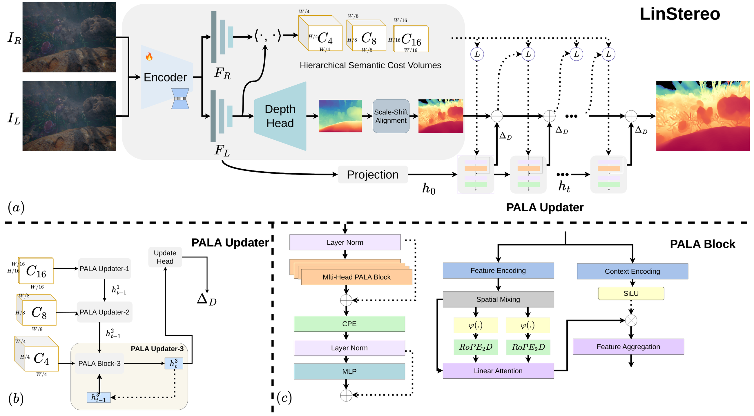
Position-Aware Linear Attention (PALA)

Standard linear attention reaches O(N) by precomputing KᵀV and sharing it across queries — but that collapses all spatial relationships into one global summary, making attention position-agnostic. PALA restores spatial structure with 2D rotary position encoding applied asymmetrically: only the numerator is position-augmented, while the denominator keeps the plain kernels for stable normalization.

O_attn = Q̃ (K̃^⊤V) · ( Q̂ K̂^⊤ + ε )⁻¹

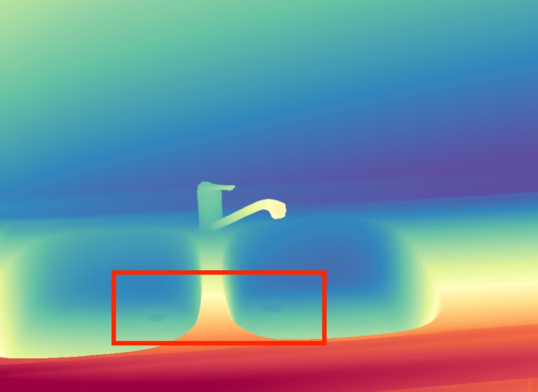
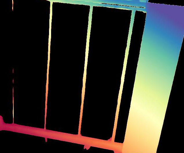
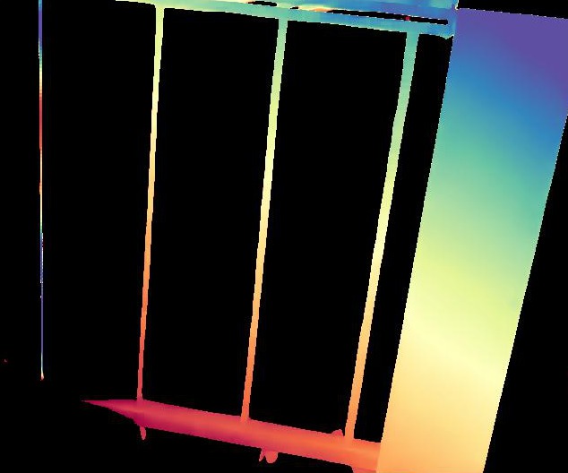
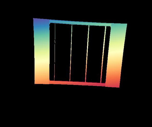
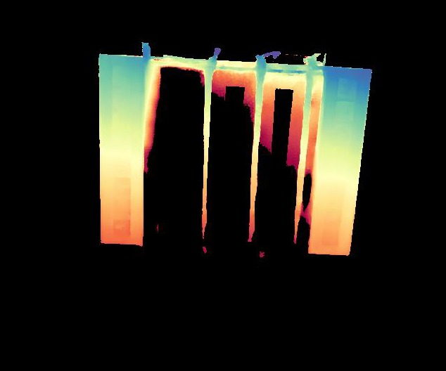
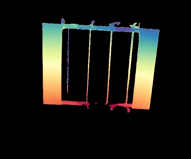
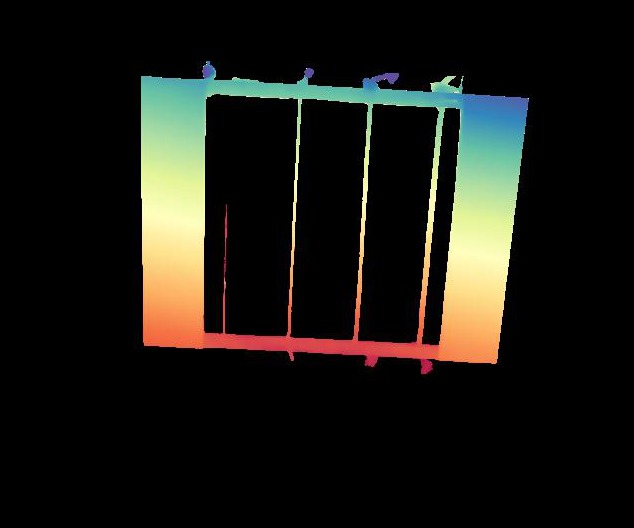
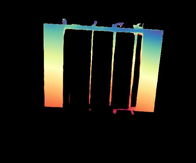
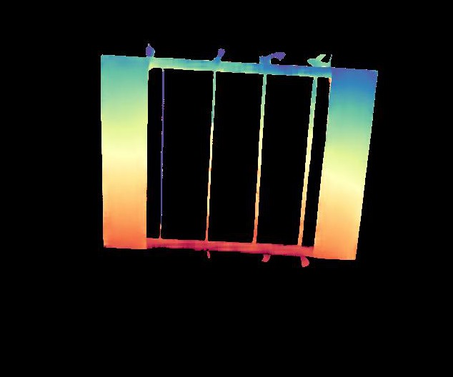
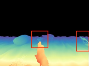
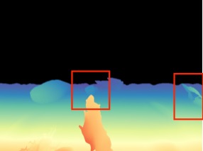
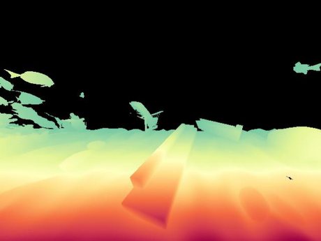
A local spatial encoding on the value branch and an adaptive gate let each location absorb new evidence where matching is confident and preserve its estimate where it is not — so reliable disparity gradually fills uncertain regions. Cost stays O(N·C²); one PALA iteration is as cheap as a ConvGRU step (3.50 ms vs 3.63 ms).

02

Hierarchical Semantic Cost Volumes (HSCV)

Instead of one fixed-resolution correlation volume, HSCV builds one per VFM scale and keeps the whole set accessible, so PALA can re-query any scale at every iteration. Each volume carries its own disparity-axis pyramid for coarse-to-fine matching while preserving spatial resolution — a two-level hierarchy across scales and within each scale.

Replacing the hierarchy with a single pooled feature degrades EPE 1.01→1.07.

03

Depth Prior Initialization (DPI)

Disparity is inversely proportional to depth, so DPI converts the monocular prediction via d = α/D_mono + β, solving the scale–shift (α,β) by least squares from sparse SIFT correspondences along epipolar lines. Refinement starts from a geometrically plausible state rather than zero.

Honest fallback: when inliers < 20 it reverts to zero-disparity init — firing on 0% of TartanAir-UW and 3.7% of SQUID frames, costing only +0.08 px EPE.

Qualitative comparison

On well-conditioned scenes recent methods look near-identical; underwater, the differences explode. The win parses in under a second.

Standard-benchmark qualitative comparison on Booster and ETH3D. — **Standard benchmarks (Booster Q & ETH3D).** LinStereo recovers sharper thin structures and handles non-Lambertian surfaces (transparent bottles, car windows).

More qualitative results

Per-benchmark comparisons, one scene per row: the input alongside recent baselines and LinStereo (Ours, highlighted) — across standard, underwater, real-world, and synthetic domains.

Standard benchmarks

Booster Input — **Booster (Q).** Transparent glass bottles, a specular metallic sink, and reflective appliances — the target depth is the physical surface, not what is seen through the glass. Baselines bleed depth around glass and leave noise on specular metal; LinStereo recovers clean contours and consistent surface depth (red boxes).

Booster IGEV++ — **Booster (Q).** Transparent glass bottles, a specular metallic sink, and reflective appliances — the target depth is the physical surface, not what is seen through the glass. Baselines bleed depth around glass and leave noise on specular metal; LinStereo recovers clean contours and consistent surface depth (red boxes).

ETH3D Input — **ETH3D.** Industrial interiors with thin pipes, low-light building exteriors, and dense outdoor vegetation. Baselines lose thin-structure continuity and produce large-area errors in dark regions; LinStereo preserves fine detail and stays stable under low light.

ETH3D IGEV++ — **ETH3D.** Industrial interiors with thin pipes, low-light building exteriors, and dense outdoor vegetation. Baselines lose thin-structure continuity and produce large-area errors in dark regions; LinStereo preserves fine detail and stays stable under low light.

KITTI 2012 Input — **KITTI 2012.** Four street scenes. LinStereo yields sharper vehicle boundaries and preserves thin structures — poles, traffic signs — that competing methods blur or fragment (red boxes).

KITTI 2012 FoundationStereo — **KITTI 2012.** Four street scenes. LinStereo yields sharper vehicle boundaries and preserves thin structures — poles, traffic signs — that competing methods blur or fragment (red boxes).

KITTI 2015 Input — **KITTI 2015.** LinStereo recovers small distant objects and road-level structure such as guard rails that the baselines over-smooth or miss (red boxes).

KITTI 2015 IGEV++ — **KITTI 2015.** LinStereo recovers small distant objects and road-level structure such as guard rails that the baselines over-smooth or miss (red boxes).

Underwater, real-world & synthetic

TartanAir-UW Input — **TartanAir-UW ①.** Simulated underwater scenes (rocky seafloor, an underwater cliff, a coral reef). Baselines overestimate depth in backscatter-affected distant regions and lose small foreground objects; LinStereo preserves accurate near-to-far transitions and resolves individual object depth.

TartanAir-UW FoundationStereo — **TartanAir-UW ①.** Simulated underwater scenes (rocky seafloor, an underwater cliff, a coral reef). Baselines overestimate depth in backscatter-affected distant regions and lose small foreground objects; LinStereo preserves accurate near-to-far transitions and resolves individual object depth.

SQUID Input — **SQUID (real-world).** Shallow sandy seafloor, near-field coral and rock, man-made equipment. Under strong color attenuation the baselines show depth-scale inconsistencies and bleeding; LinStereo keeps stable depth and recovers fine detail. Black = unavailable depth.

SQUID FoundationStereo — **SQUID (real-world).** Shallow sandy seafloor, near-field coral and rock, man-made equipment. Under strong color attenuation the baselines show depth-scale inconsistencies and bleeding; LinStereo keeps stable depth and recovers fine detail. Black = unavailable depth.

Real-world tank Input — **Real-world lab tank — close-up.** A controlled water tank imaged at close range (< 2 m) with AprilTag + CAD-model ground truth down to sub-millimetre, including ~3 mm taut ropes as a fine-structure stress test. Columns: left, right, GT, then five baselines and **Ours**. LinStereo resolves the thin ropes and tank geometry that baselines blur, fragment, or miss. Black = no valid GT.

Real-world tank Right — **Real-world lab tank — close-up.** A controlled water tank imaged at close range (< 2 m) with AprilTag + CAD-model ground truth down to sub-millimetre, including ~3 mm taut ropes as a fine-structure stress test. Columns: left, right, GT, then five baselines and **Ours**. LinStereo resolves the thin ropes and tank geometry that baselines blur, fragment, or miss. Black = no valid GT.

SeaStereo Input — **SeaStereo (synthetic).** Left, right, ground truth, then five baselines and **Ours**, across Jerlov water types. Baselines show edge noise or shape distortion on elongated structures and over-smooth vegetation, losing depth layering; LinStereo preserves sharp object contours and foreground–background separation.

SeaStereo Right — **SeaStereo (synthetic).** Left, right, ground truth, then five baselines and **Ours**, across Jerlov water types. Baselines show edge noise or shape distortion on elongated structures and over-smooth vegetation, losing depth layering; LinStereo preserves sharp object contours and foreground–background separation.

Reproduced from the paper's supplementary material. See the paper for full discussion.

SeaStereo Dataset

A physically-rendered underwater stereo corpus with dense disparity ground truth, released with the paper.

~40Kstereo pairs

7Jerlov water types

1000+configurations

denseGT disparity

SeaStereo rendering pipeline: ShapeNet objects composited over marine backgrounds in Blender under Jerlov water models. — **Rendering pipeline.** ShapeNetCore foreground objects composited over real marine backgrounds (coral, fish, shipwrecks) and rendered in Blender under varying Jerlov water types — spanning 1000+ configurations with varied trajectories, focal lengths, inter-ocular distances, and seafloor depths.

More dataset samples

Each card shows the left & right stereo views and the dense disparity ground truth, spanning Jerlov water types I–3C, seafloor depths, and camera configurations.

LeftRightDisp.

Jerlov IA · shallow

LeftRightDisp.

Jerlov IB · shallow

LeftRightDisp.

Jerlov IC · shallow

LeftRightDisp.

Jerlov 3C · shallow

LeftRightDisp.

Jerlov IB · shallow

LeftRightDisp.

Jerlov II · shallow

LeftRightDisp.

Jerlov III · shallow

LeftRightDisp.

Jerlov I · deep

LeftRightDisp.

Jerlov II · deep

LeftRightDisp.

Jerlov I · deep

LeftRightDisp.

Jerlov IA · deep

LeftRightDisp.

Jerlov IB · shallow

Download SeaStereo soon

Water-condition explorer

Hold the method fixed, change the water. As turbidity and depth climb, LinStereo holds.

LinStereo result under varying water conditions

Standard benchmarks

Zero-shot cross-domain, official weights. We keep LinStereo a ViT-B, SceneFlow-only model to isolate the decoder's contribution — competitive with ViT-L systems and extra-data methods, and best among comparable models on occluded Middlebury.

Method	Extra data	KITTI 2015		KITTI 2012		Middlebury (H)						ETH3D		Booster (Q)
Method	Extra data	EPE↓	bad3↓	EPE↓	bad3↓	All EPE↓	All bad2↓	Noc EPE↓	Noc bad2↓	Occ EPE↓	Occ bad2↓	EPE↓	bad1↓	EPE↓	bad2↓
PSMNet	–	4.05	28.51	3.77	27.34	11.48	36.06	10.56	32.11	17.69	62.58	2.15	15.13	14.17	49.79
RAFT-Stereo	–	1.13	5.69	0.90	4.35	1.92	12.6	1.09	8.65	3.31	26.39	0.36	3.3	4.18	17.64
IGEV-Stereo	✓	1.21	6.03	1.03	5.13	2.63	11.93	2.27	9.49	5.02	26.04	0.33	4.0	4.26	17.58
UniMatch	–	1.63	11.01	1.71	12.04	4.21	34.72	3.96	31.52	5.70	56.51	0.69	18.61	8.57	47.30
Selective-RAFT	✓	1.27	6.68	1.08	5.19	2.34	12.04	2.05	9.45	4.17	27.4	0.34	4.36	4.14	19.52
Selective-IGEV	✓	1.25	6.06	1.08	5.64	2.59	11.79	2.31	9.22	4.35	28.10	0.33	4.05	4.62	19.28
MoCha-Stereo	–	1.29	5.97	1.02	4.83	2.66	10.18	2.49	7.96	3.84	24.16	0.28	3.47	3.88	16.82
NMRF	–	1.17	5.31	0.92	4.63	2.91	13.36	2.73	10.90	4.22	29.27	0.31	3.8	5.05	26.22
IGEV++	✓	1.27	6.22	1.20	6.81	3.21	10.85	2.41	7.86	6.83	28.68	0.35	4.60	5.00	18.62
MGStereo	–	1.13	5.62	0.87	4.16	1.15	8.39	0.85	5.67	2.89	26.50	0.25	1.88	2.26	11.02
Stereo Anywhere ViT-L	–	1.07	4.93	0.83	3.90	0.94	6.96	0.79	4.75	2.67	20.34	0.24	2.66	2.21	9.91
DEFOM-Stereo ViT-L	–	1.06	4.99	0.84	3.76	0.84	5.91	0.90	5.76	2.11	19.34	0.35	2.35	3.52	13.20
MonSter ViT-L	–	0.89	3.58	0.75	3.58	1.98	10.41	2.03	8.79	2.62	21.56	0.23	1.41	3.08	17.45
BridgeDepth ViT-L	–	1.13	4.90	0.86	4.39	2.21	10.27	2.25	8.66	2.68	20.42	0.24	1.33	4.71	18.79
FoundationStereo ViT-L	✓	0.95	3.65	0.71	3.18	0.71	3.47	0.42	1.46	2.67	16.44	0.21	1.14	1.77	6.89
LinStereo ViT-B (Ours)	–	1.01	4.54	0.76	3.49	0.83	6.01	0.89	5.67	1.33	8.69	0.24	2.41	2.14	9.93

Bold = best, underline = second-best among comparable methods (no extra data). FoundationStereo (ViT-L + extra data, grey) is the strongest baseline overall and shown for reference. LinStereo's 1.33 occluded-EPE on Middlebury is 37% below the previous best (DEFOM, 2.11) — direct evidence of PALA propagating reliable disparity into occluded pixels. EPE and badX (% pixels past the error threshold) reported per benchmark; scroll the table sideways for all columns.

Underwater generalization

The headline domain. Trained on SceneFlow only, LinStereo is best on every metric on both benchmarks — even against methods trained with real-world or domain-specific data.

Method · TartanAir-UW (simulated, long-range backscatter)	Extra data	AbsRel↓	SqRel↓	RMSE↓	LogRMSE↓	A1↑	A2↑	A3↑
UniMatch	–	0.17	2.59	6.35	0.26	0.759	0.830	0.837
MoCha-Stereo	–	0.15	2.30	6.02	0.25	0.769	0.835	0.843
NMRF	–	0.11	1.08	4.63	0.21	0.811	0.856	0.870
PSMNet	–	0.10	1.02	4.56	0.21	0.813	0.857	0.871
RAFT-Stereo	–	0.08	0.65	4.36	0.20	0.902	0.963	0.984
MGStereo	–	0.08	0.55	3.69	0.19	0.911	0.968	0.987
Stereo Anywhere	–	0.06	0.41	3.24	0.18	0.946	0.980	0.989
DEFOM-Stereo	–	0.05	0.41	3.13	0.17	0.953	0.982	0.990
Selective-Stereo (RAFT)	✓	0.09	0.67	4.31	0.21	0.902	0.962	0.981
Selective-Stereo (IGEV)	✓	0.11	1.02	5.01	0.23	0.856	0.942	0.976
IGEV-Stereo	✓	0.10	0.90	4.68	0.21	0.891	0.955	0.979
IGEV++	✓	0.09	0.81	4.37	0.20	0.905	0.962	0.983
FoundationStereo	✓	0.05	0.40	3.01	0.16	0.959	0.984	0.991
LinStereo ViT-B (Ours)	–	0.04	0.19	2.08	0.09	0.959	0.992	0.998

Method · SQUID (real-world, color attenuation)	Extra data	AbsRel↓	SqRel↓	RMSE↓	LogRMSE↓	A1↑	A2↑	A3↑
UniMatch	–	1.38	20.91	6.42	0.66	0.561	0.660	0.734
MoCha-Stereo	–	0.15	0.61	1.55	0.20	0.875	0.931	0.958
NMRF	–	0.43	5.27	2.57	0.33	0.844	0.904	0.935
PSMNet	–	0.46	4.31	3.43	0.51	0.736	0.813	0.853
RAFT-Stereo	–	0.07	0.27	1.25	0.12	0.937	0.971	0.987
MGStereo	–	0.09	0.71	1.99	0.16	0.925	0.958	0.976
Stereo Anywhere	–	0.07	0.40	1.46	0.13	0.937	0.976	0.985
DEFOM-Stereo	–	0.09	0.63	2.00	0.16	0.915	0.954	0.977
Selective-Stereo (RAFT)	✓	0.11	0.22	1.16	0.16	0.877	0.940	0.968
Selective-Stereo (IGEV)	✓	0.08	0.21	1.05	0.14	0.932	0.966	0.980
IGEV-Stereo	✓	0.20	1.35	2.68	0.46	0.760	0.821	0.863
IGEV++	✓	0.06	0.22	1.11	0.12	0.950	0.981	0.990
FoundationStereo	✓	0.07	0.30	1.36	0.13	0.940	0.976	0.987
LinStereo ViT-B (Ours)	–	0.04	0.12	0.90	0.08	0.970	0.990	0.996

The largest gains track each benchmark's dominant degradation: 31% lower RMSE than FoundationStereo on TartanAir-UW (long-range backscatter) and 26% lower AbsRel than IGEV++ on SQUID (color attenuation). All baselines shown; AbsRel/SqRel/RMSE/LogRMSE lower is better, A1/A2/A3 higher is better.

Real-world deployment

Beyond simulation: a controlled laboratory water tank at close range (< 2 m), with AprilTag + CAD-model ground truth down to sub-millimetre — including ~3 mm taut ropes as a fine-structure stress test.

Method	Extra data	AbsRel↓	SqRel↓	RMSE↓	LogRMSE↓	A1↑	A2↑	A3↑
PSMNet	–	0.18	0.16	0.34	0.28	0.87	0.90	0.93
UniMatch	–	0.08	0.04	0.17	0.16	0.93	0.96	0.98
Stereo Anywhere	–	0.09	0.06	0.20	0.19	0.92	0.93	0.97
RAFT-Stereo	–	0.06	0.03	0.15	0.14	0.94	0.96	0.99
MGStereo	–	0.08	0.05	0.18	0.17	0.93	0.94	0.98
Selective-Stereo (RAFT)	✓	0.07	0.03	0.14	0.14	0.94	0.97	0.99
Selective-Stereo (IGEV)	✓	0.08	0.04	0.16	0.16	0.91	0.95	0.99
IGEV-Stereo	✓	0.06	0.02	0.13	0.12	0.94	0.97	0.99
IGEV++	✓	0.05	0.02	0.12	0.12	0.96	0.97	0.99
FoundationStereo	✓	0.07	0.04	0.18	0.17	0.93	0.94	0.98
LinStereo (Ours, T=8)	–	0.04	0.01	0.07	0.07	0.98	0.99	1.00

Bold = best. Extra data (✓) = trained beyond SceneFlow. AbsRel/SqRel/RMSE/LogRMSE lower is better; accuracy thresholds A1/A2/A3 higher is better. Scored only on valid-GT pixels projecting onto the CAD mesh. LinStereo — SceneFlow-only — leads every metric at this near-range, fine-structure target. Qualitative close-up in More qualitative results → Real-world tank.

Efficiency & runtime

LinStereo trades raw speed for accuracy and zero-shot generalisation: it is a large model built on a frozen Depth Anything V3 backbone. The cost is explicit below — yet its core PALA update operator costs about the same per iteration as a local ConvGRU, despite being global and linear in image size.

Computational efficiency

Method	Params (M)↓	GFLOPs↓	Time (ms)↓	FPS↑
LightStereo-S	3.44	45.4	9.9	101.0
CoEx	2.73	70.6	11.0	91.0
CGI-Stereo	3.50	81.6	12.8	78.1
Fast-ACVNet	3.08	104.6	13.2	76.0
ADStereo	7.10	201.6	15.4	64.7
RAFT-Stereo†	9.87	296.4	18.0	55.7
RT-IGEV	4.17	354.2	24.7	40.5
MobileStereoNet	2.35	175.6	37.7	26.5
AANet	3.93	–	65.8	15.2
LinStereo (Ours, T=2)	127.0	770.4	80	12.5

Bold = best. Measured at 480×640 on a single NVIDIA RTX 4500 (24 GB); LinStereo at T = 2 (accuracy elsewhere uses T = 8). LinStereo is a large, accuracy-first model — not a lightweight real-time network.

Per-iteration update operator

Update operator	Latency (ms)↓
PALA (Ours)	3.50 ± 0.05
RAFT-Stereo ConvGRU	3.63 ± 0.06
IGEV ConvGRU	3.43 ± 0.03

Per-update latency at 480×640 (± 95% CI). PALA's global, linear-complexity attention costs essentially the same per iteration as the local ConvGRU operators it replaces.

BibTeX

@inproceedings{wang2026linstereo,
  title         = {LinStereo: Linear-Complexity Global Attention for
                   Multi-Scale Iterative Stereo Matching},
  author        = {Wang, Yiran and Turner, Oliver and Ila, Viorela},
  booktitle     = {European Conference on Computer Vision (ECCV)},
  year          = {2026},
  eprint        = {2606.25437},
  archivePrefix = {arXiv},
  primaryClass  = {cs.CV}
}

LinStereo

Drag to reveal

Abstract

Method

HSCV

DPI

PALA

Position-Aware Linear Attention (PALA)

Hierarchical Semantic Cost Volumes (HSCV)

Depth Prior Initialization (DPI)

Qualitative comparison

More qualitative results

Standard benchmarks

Booster

ETH3D

KITTI’12

KITTI’15

Underwater, real-world & synthetic

TartanAir-UW ①

TartanAir-UW ②

SQUID

Real-world tank

SeaStereo

SeaStereo Dataset

More dataset samples

Water-condition explorer

Standard benchmarks

Underwater generalization

Real-world deployment

Efficiency & runtime

Computational efficiency

Per-iteration update operator

BibTeX